8 Setting up landscapes
Initialization of a simulation landscape in iLand entails four core components:
Landscape and forest extent (Section 8.1)
Geospatial data on biophysical drivers (Section 8.2)
Initial vegetation conditions (Section 8.3)
Information about disturbance regimes and/or management (Section 8.4)
Although initialization typically refers to simulating landscapes that represent real locations, iLand is also used to simulate individual stands (Hansen et al. 2020; Kobayashi et al. 2023) or generic, hypothetical landscapes (Braziunas et al. 2018) depending on the research questions.
8.1 Landscape extent
Landscape extents often align with jurisdictional boundaries, natural barriers to seed dispersal, or disturbances such as ridge tops or large water bodies, or the edges of an entire forest patch. Once boundaries are defined, forested or potentially forested (i.e., stockable) area must be further delineated within the landscape, because iLand is specifically designed to simulate forest dynamics and doesn’t explicitly represent vegetation types that would prevent forest expansion into non-forested areas. Stockable area in iLand landscapes typically ranges in the 1,000s to 10,000s of ha, although the landscape extent may be much larger if there are extensive non-forested areas.
This chapter explains how to set up a “real” landscape. Information on other types of simulation set-ups (e.g., for growth evaluation tests) can be found here.
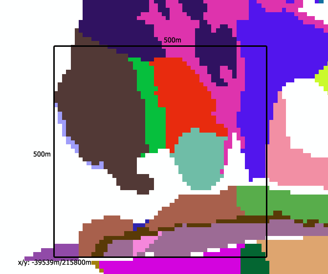
8.1.1 Stand grid
The stand grid is the definition of the project area as a GIS grid (10m resolution). It is often derived from polygonal data, e. g., a map of stand polygons. The stand grid defines the forested area of the project landscape and the spatial distribution of forest stands within it at the beginning of the simulation. Stand delineation is often based on the forest management history (stands as management units) or forest type maps (stands as forest patches with similar composition and structure). A stand is defined by an integer ID greater than zero. Cells with the same grid value belong to the same “stand”. In addition to the forested area within the project area, the grid contains information about the area surrounding the forest:
Pixel values of -1 (or the NO_DATA_VALUE of the grid) = “non-forested outside pixel”: non-project-area, no regeneration establishment possible
Pixel values of -2 = “forested outside pixel”: continuous “shading” from the assumed forest outside of the project area is applied (LIF calculation), can act as source of external seeds, included in fetch calculations of the wind module
The stand grid can also be used to initialize the tree vegetation of each stand (see Initializing with forest inventory data).
8.2 Biophysical landscape
The next step after defining the size and the boundaries of the project area is to define the actual content, i.e. the distribution of biophysical drivers like topography, daily climate data, and soil properties atop of the landscape. Their distribution is initialized in iLand via the environment file and grid, which define site and climate conditions:
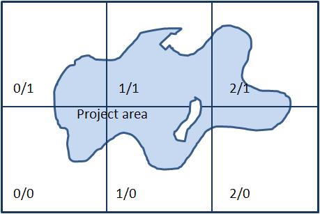
The environment grid contains regions with homogeneous soil and climate conditions with a resolution of 100m (these cells are henceforth referred to as resource units). The grid itself holds an (integer) “id” for these units
The environment file is a table (CSV or other text format) containing for each “id” (i.e., resource unit) the values for soil and climate conditions (and also things like carbon pools for soil and deadwood)
When iLand initializes a resource unit, it uses the values provided in the environment file. The environment file can also be used to establish a link to climate data (see Climate). Each row contains the information about one resource unit:
| Key (column name in the environment file) | Description |
|---|---|
| id | resource unit id corresponding to the environment grid (grid mode) |
| x | 0-based index of the resource unit in x-direction (matrix mode) |
| y | 0-based index of the resource unit in y-direction (matrix mode) |
| model.site.availableNitrogen | available nitrogen of the unit (kg/ha/yr) |
| model.site.soilDepth | depth of soil (cm) of the unit |
| model.site.pctSand, model.site.pctSilt, model.site.pctClay (one column each) | soil texture [%], cell-wise sum = 100 |
| model.climate.tableName | climate data for that unit (table name in the .sqlite-file) |
If the environment file does not contain a specific key, then the value provided in the project file is used throughout the landscape. The keys refer to nodes in the project file. More keys can be added if needed (e.g., keys for Dynamic carbon cycling or Fire).
8.2.1 Topography
Topographic drivers used in iLand are derived from digital elevation models (DEM), which are often available at high resolution across the globe (e.g., the US National Elevation Dataset, Germany Digital Terrain Models). The resolution of the input file may vary, and iLand internally creates a DEM with a resolution of 10 m and calculates maps of slope and aspect. The DEM is optional and doesn’t affect simulation outcomes. When no DEM is given, a flat topography is assumed.
8.2.2 Climate
Daily climate data for the time period of interest (e.g., historical, future) and required variables (global radiation, minimum and maximum temperature, precipitation, vapor pressure deficit) is often available at regional, continental, or global scales, although spatial resolution and availability of specific future climate models may vary. Additional steps can be taken to downscale daily climate to the resolution of resource units in iLand (Thom et al. 2022) or generate daily time series from coarser temporal resolutions. Annual atmospheric CO2 concentration can also be incorporated as a climate driver.
Data about daily climate is stored in SQLite-databases which contain one table per climate cluster. Climate clusters are regions of the landscape with similar climatic conditions and are independent of the stand grid. Each resource unit is assigned to one climate cluster (table in the climate-SQLite). The link between resource unit and climate table is established in the environment file (key “model.climate.tableName”, see Biophysical landscape). Climate scenarios (“historic”, “RCP85” etc.) are stored in separate .sqlite-files.
8.2.2.1 Downscaling climate data
Since future climate models are most commonly available only at resolution coarser than 100 m, methods for downscaling climate data have been developed. This is especially important in topographically complex landscapes. The method leverages the relationship between climatic variables (especially temperature and precipitation) and elevation. The lapse rate (the rate at which a climate variable changes with elevation) is calculated for each climate variable and then used for downscaling each 100x100 m-cell’s climate parameters based on the cell’s elevation. The method has been successfully applied in Thom et al. (2022) . The pipeline for the method is available on request from Christina Dollinger.
8.2.3 Soil properties
Soil properties including soil depth, texture, plant available nitrogen, and, if the carbon cycle is enabled, carbon pools tend to be more challenging to obtain. Spatially explicit maps of soil properties may be available only at local to regional scales or may not exist. A categorical soil type map is often used in combination with ancillary data such as soil samples, forest type, or forest productivity to estimate and assign average soil properties. Global soil databases are becoming increasingly available (Poggio et al. 2021), but may not include all variables and vary in accuracy across regions. If soil carbon or nitrogen cycling is enabled, a spin-up process can be used to derive initial pools (Hansen et al. 2020).
The minimal setup of soil properties includes spatially explicit data on soil texture (the percentage of sand/silt/clay), effective soil depth (cm), and available nitrogen (kg/ha/year) for the landscape. The soil properties of each resource unit are specified in the environment file (keys “model.site.pctSand” / “model.site.pctSilt” / “model.site.pctClay” / “model.site.soilDepth” / “model.site.availableNitrogen”, see Biophysical landscape).
8.2.3.1 Dynamic soil carbon cycling
iLand uses the ICBM/2N model (Kätterer and Andrén 2001) to model the C in dead organic matter and soil pools. The technical implementation follows these steps:
Obtain initial values for the carbon pools: spatially explicit data about coarse woody debris carbon pools (“model.site.youngRefractoryC” in the environment file), litter carbon pools (“model.site.youngLabileC”) and soil organic matter carbon pools (“model.site.somC”)
Dynamically calculate the influx rates of dead organic matter:
Simulate the landscape for 200 years, with carbon pools initialized with the values stated above
Extract the annual fluxes of dead organic matter simulated by iLand for each 100x100 m-cell in the last 50 years of simulation from the output “soilinput” (input_lab and input_ref and the aboveground fractions input_lab_ag, input_ref_ag)
Calculate mean decomposition rate of litter and coarse woody debris over the whole landscape (species parameter “snagKyl” and “snagKyr” in the species table)
Calculate the decomposition rate of soil organic material for each resource unit using the humification rate (either based on literature or estimated by running a sensitivity analysis)
More information on the description of the C model can be found here and on the parametrization process here.
8.3 Vegetation
Initial vegetation consists of species- and size-specific data on live individual trees and regeneration cohorts. Dead vegetation (e.g., snags, downed wood) can also be initialized. Forest inventory plots in combination with spatially continuous data such as canopy height from LiDAR or interpolation or imputation methods (e.g., FIA plot imputation by Riley, Grenfell, and Finney (2016)) can enable detailed wall-to-wall representations of current forest structure and composition. Alternatively, approximate forest conditions can be generated using a customizable spin-up process. The spin-up process ranges from potential natural vegetation, in which simulations start from bare ground with seed inputs from the landscape edge and run for 100s to 1,000s of years (Albrich, Rammer, and Seidl 2020), to a directed spin-up, in which target values such as stand age, tree size distributions, and composition are set and simulations are run iteratively until the realized conditions are close to expected values (Dobor et al. 2020).
8.3.1 Initializing with forest inventory data
Forest inventory data or data from independent field work can be used to initialize vegetation. For each stand (see Stand grid) information about stem density, tree species and DBH distributions is needed. This data is compiled in an “initialization file” (node model.initialization.file in the project file). Each line in the input file describes a number of trees (count) of a certain species. The diameter is randomly chosen from the range dbh_from and dbh_to. The height is calculated using the defined height/diameter ratio (hd). All trees of this class have the same age:
| Column | Description |
|---|---|
| count | number of trees per hectare |
| species | the alphanumeric code of the tree species (e.g. piab, fasy) |
| dbh_from, dbh_to | the range of diameters (cm) for the trees. For each tree, the actual diameter is chosen from a uniform random distribution. |
| hd | height-diameter relation (m/m). The height of each tree is calculated as dbh*hd |
| age | (optional) age of the trees (years). If blank or zero the age is estimated. |
| density | (optional) density value ranging from -1..1 (see description below). Default=0. |
| stand_id | indicates the stand in standgrid mode. |
Within a stand the positions of the individual trees are derived by applying an pseudo-random approach (more information here) but can also be set using the single tree initialization approach (more information here).
The same approach can be used to initialize saplings (i.e. trees < 4m, see here).
8.3.2 Spin-up
After initializing vegetation a spin-up is run to reach a vegetation state as close as possible to the reference data while also ensuring that the initial state is consistent with model logic (e.g. tree placement, competition effects). The model is run under an approximation of past climate and disturbances (and past management if applicable) for multiple centuries. Spin-ups vary in length and should consider the target age of the oldest forest stands and the timescales needed to represent forest processes, such as decomposition and soil carbon cycling if these processes are enabled. In landscapes where disturbance or management play a pivotal role in shaping forest conditions, historical disturbance or management regimes can be simulated during the spin-up. Furthermore, actual disturbance events or management activities can be spatially and temporally explicitly prescribed (e.g., real fire perimeters are used in the spin-up in Turner et al. (2022)).
A more elaborate spin-up procedure is the directed spin-up. Here the end state of the spin-up is not determined by a simulation length or simultaneously for the whole landscape but rather based on how well each stand corresponds with reference conditions at the given age (Thom et al. 2018).
A spin-up can also be run without previous vegetation initialization and instead starting from bare ground with external seed inputs (“potential natural vegetation” run). There are multiple options for simulating external seed input (see External seed input).
The final vegetation state of the spin-up is then saved as a “snapshot”. A snapshot is a full representation of the internal vegetation and soil state of a landscape and is stored in a database. This snapshot can later be used to restore a previous vegetation state. The snapshot includes all state variables of trees, saplings, snags and soil-pools. A snapshot is created by using the JavaScript function saveModelSnapshot(). This function creates a SQLite database file (which can be quite large) and an additional resource-unit map as a ESRI raster-file with the same name (and .asc as file extension).
To load a snapshot, one can use the mode “snapshot” in the project-file for the tree initialization (nodes world.initialization.mode and world.initialization.file in the project file). More information on snapshots can be found here.
8.3.3 External seed input
Especially for “bare ground”/PNV runs but also for other purposes it can be useful to provide the landscape with a continuous input of seeds generated outside of the landscape. Two distinct approaches exist: the “seed belt” approach simulates seed input from forests outside of the landscape, while the “seed rain” approach provides the whole area of the landscape with a continuous supply of seeds.
The next sections give an overview of the two approaches, more detail on their implementation can be found here.
8.3.3.1 Seed belt
The seed belt is a belt shaped area surrounding the project area. This belt acts as a seed source and seeds reach the project area from the belt facilitating the iLand seed dispersal algorithm. The total area is split into a number of sectors, whereas each sector is characterized by an user-defined species composition. The seed belt is limited to those areas outside of the project area that are flagged as “forested” (pixel values of -2, see Stand grid).
The number of sectors, as well as each sector’s unique mix of seeds differing in species and seed share (0-1) can be defined in the project file.
The following snippet is an example for defining the seed belt in the project file:
<seedBelt>
  <enabled>true</enabled>
    <width>9</width>
    <sizeX>3</sizeX>
    <sizeY>2</sizeY>
    <species_0_0>Abam 0.7 Psme 0.1</species_0_0>
    <species_0_1>Psme 0.1</species_0_1>
    <species_1_1>Psme 0.1</species_1_1>
    <species_2_1>Psme 0.1</species_2_1>
</seedBelt>
Example how a seed belt can be defined in the project file
8.3.3.2 Seed rain
In some cases, it could be useful to have external seed input on the full area, i.e., on all pixels regardless of their location. In the project file a list of species and their seed availability probability can be specified, for example: “piab, 0.01, fasy, 0.02, bepe, 0.03”. This sets the seed probability of Norway spruce (piab, the species shortName in the species parameter table) to 0.01, of beech to 0.02 and of silver birch to 0.03. The probability is interpreted as the chance of having no seed limitation on each 2x2m cell (e.g., a value of 0.01 would mean that - in the absence of other limitations (environment, light, cell already occupied by saplings of the species) - cohorts would establish every year on roughly 1% of the 2x2m cells).
8.4 Additional steps
Finally, initialization requires information on disturbance and management regimes. Built-in abiotic and biotic disturbance modules must be parameterized to ensure appropriate representation of disturbance size, severity, and frequency (Hansen et al. 2020). Sequences of disturbance events can also be generated separately and prescribed (Albrich et al. 2022), enabling greater control in exploring variation in timing, frequency, size, or intensity among disturbance scenarios. Forest management is extremely flexible: for example, one can define thresholds that initiate actions, develop new treatment methods, include spatially explicit prioritization of management zones, or employ agent-based managers that react to their environment in dynamic and complex ways.
8.4.1 Disturbances
While some disturbance modules (e.g., bark beetle Ips typographus) are implemented in iLand fully dynamically, and thus do not need any parameterization before applying the sub-module to new situations, other disturbance modules (e.g., wind, fire) require landscape-specific information for their implementation.
8.4.1.1 Wind
The wind module in iLand (see here for more details) requires two types of landscape-specific inputs: a time series of wind events (with accompanying properties like wind direction and storm duration, see here) and a raster file at a resolution of 100x100 m which scales the global wind pattern to a local value (“topoModifier”-grid).
Data on wind speeds [m/s, measured at 10 m above ground] can for example be obtained from weather stations. Storm events are identified as the 90th percentile of yearly top wind speeds and their main wind direction is also determined. Time series of wind events can then be generated by sampling with a Gumbel distribution (Thom et al. 2022). To account for how wind speeds are modified by topography, spatial data on mean annual wind speeds is used to create the topoModifier-grid, which for each 100x100 m cell contains a value with which to modify (additive or multiplicative) the wind speed given in the time series.
Finally, simulated wind disturbance patterns need to be evaluated against data on historical wind regimes (e.g., simulated versus observed wind damage, see Thom et al. (2022)).
8.4.1.2 Fire
Parameterization and evaluation of the iLand fire module should include comparisons of simulated versus observed data to assess multiple aspects of the disturbance regime, such as fire sizes, shapes, annual area burned, and severity. The base fire module is described in detail on the wildfire module overview, fire module parameters and fire module evaluation wiki pages.
The fire module is easily customizable using additional scripts and inputs. For example, Hansen et al. (2020) included a value for KBDI (Keetch Byram Drought Index, the drought indicator used in the iLand fire module) that separated cooler-wetter from hotter-drier years. Fire sizes in iLand were assigned different minimum and maximum sizes and drawn from different fire size distributions depending on whether KBDI was above or below this threshold value. This functionality was implemented in a separate javascript. Or, Turner et al. (2022) combined iLand simulations with fire sizes generated from a separate statistical modeling process that estimated ignition locations and fire sizes under different projected future climate models. Consistent with fire sizes in the western United States, which can be 10,000s to 100,000s of ha, estimated fire sizes could be larger than an iLand landscape. In their paper, Turner et al. (2022) developed a process to first estimate how much of a potential future fire would be expected to “burn in” to a given landscape and then prescribed a distinct sequence of fire events (fire year, ignition location, and maximum size) for each future simulation replicate. This is conceptually similar to the way wind time events are implemented (described above), although in this case it was implemented via a customized JavaScript.
8.4.1.3 Bark beetle
The bark beetle disturbance module (see here for more details) does not need to be parameterized (but note that it is specific to the European spruce bark beetle). It does however need to be adapted to a new landscape using the following nodes in the project file:
modules.barkbeetle.referenceClimate.tableName
name of the table in the climate-SQLite that represent the reference climate for the landscape. iLand compares the climate values given by that table with the baseline climate values given by the project file nodes seasonalPrecipSum and seasonalTemperatureAveragemodules.barkbeetle.referenceClimate.seasonalPrecipSum
comma-delimited list of historic seasonal precipitation sums (spring, summer, autumn, winter) extracted from the climate table given in tableName. Example:212, 234, 190, 179modules.barkbeetle.referenceClimate.seasonalTemperatureAverage
comma-delimited list of historic seasonal mean temperatures extracted from the climate table given in tableName. Seasons are: spring: March, April, May, summer: June, July, August, autumn: Sept., Oct., Nov., winter: Dec., Jan., Feb. Example:7.6, 13.2, 6.9, 3.3
For more information on the parameterization of the bark beetle module see Seidl and Rammer (2017) .
8.4.1.4 BITE
The Biotic Disturbance Engine (or BITE, see here) can simulate biotic disturbances in forest ecosystems. Its framework is also simple, modular and general enough to simulate a wide range of biotic disturbance agents, from fungi to large mammals. More information can be found in Honkaniemi, Rammer, and Seidl (2021) .
8.4.2 Management
If the landscape of interest had been shaped by management in the past, it is recommend to mimic these interventions in the spin-up to generate representative forest states. Two modules for management are integrated in iLand: the base management module (see here) and the Agent Based management Engine (ABE, see here), with the latter one being able to simulate adaptive forest management in multi-agent landscapes. More details on the management modules can be found in the Forest management chapter.