10 Calibration and evaluation of species and simulation results
Once species are parameterized, the next steps are calibration and evaluation. This is an iterative process. When evaluations highlight discrepancies between simulations and comparison data, parameters can be changed, or calibrated, to improve evaluation outputs and model fit (see examples of parameters to focus on here and in sections below). It is important to think critically, and ecologically, about the evaluation experiments during this process. Model fits should not be expected to be perfect; data inputs such as climate and soils have inherent uncertainty or simplification, some processes such as disturbances are not represented in the basic evaluations, and comparison datasets may have their own biases (e.g., site indexes are idealized curves, forests may have unknown management history or be influenced by unmeasured neighboring stands). The evaluations should help you build confidence that the model is representing processes of productivity and growth, mortality, regeneration, and competition in a way that aligns with available data and your ecologically-informed expectations.
There are several options for evaluating iLand’s ability to simulate realistic forest growth and composition patterns. Evaluation tests encompass different hierarchical levels (individual, stand, and landscape; see Table 10.1) following a pattern-oriented approach (Grimm et al. 2005) and are usually run under historical climate conditions. The suite of evaluation tests has to be designed carefully for each project as there is no one-size-fits-all approach (e.g., due to limited data availability). This section gives an overview of the types of tests used in previous studies, their data requirements, simulation set-up, calibration recommendations, and evaluation strategy.
Included in this process are the iterative calibration of some species parameters that are derived from model simulations, rather than the literature (see also Species parameter chapter).
| Hierarchical level | Evaluation target |
|---|---|
| Individual-tree level |
|
| Stand level |
|
| Landscape level |
|
The examples below are grouped by ecological processes and parameter tier, which include evaluations at different hierarchical levels.
10.1 Productivity and mortality
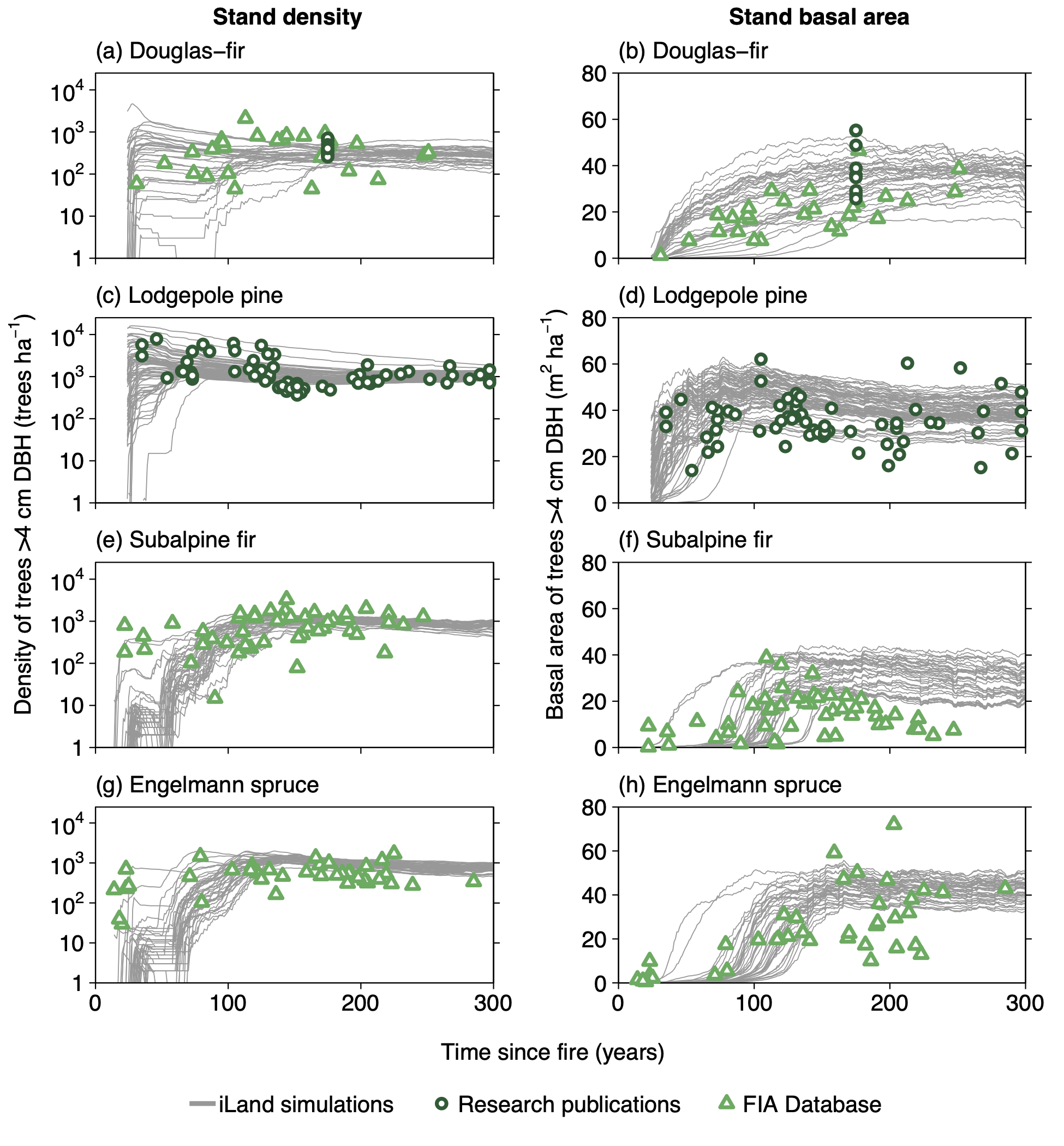
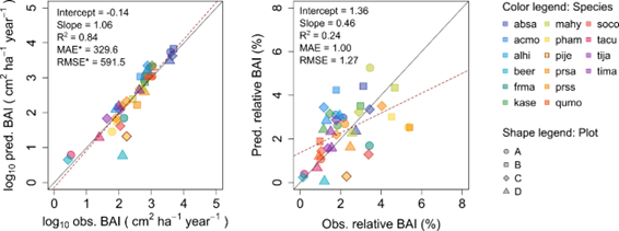
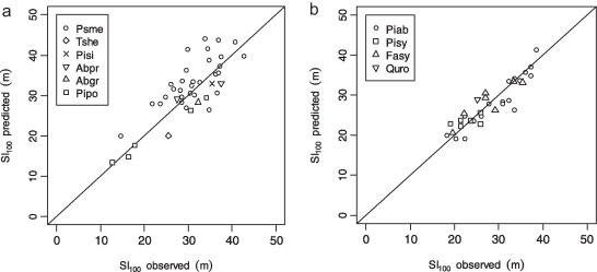
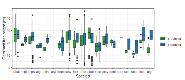
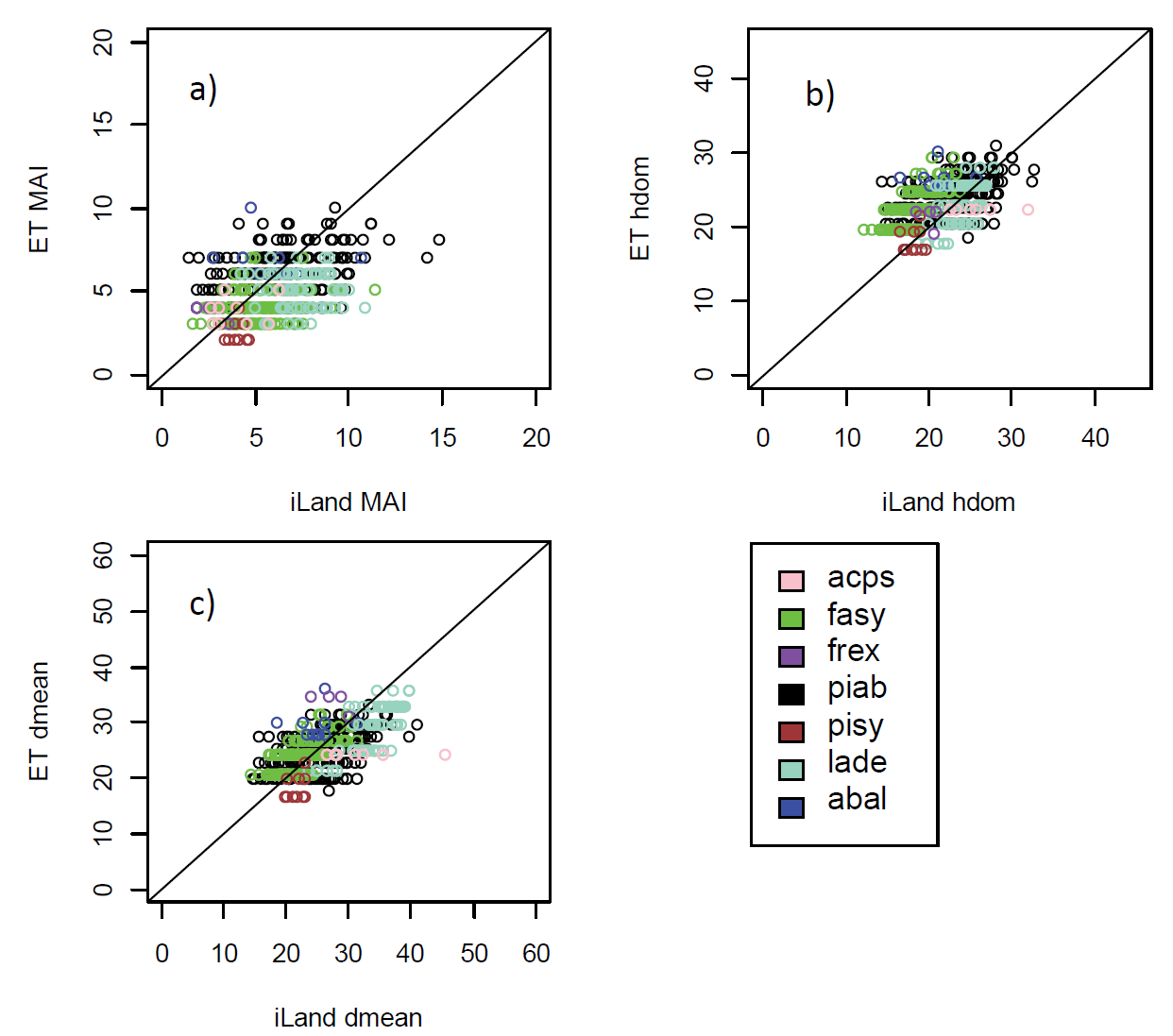
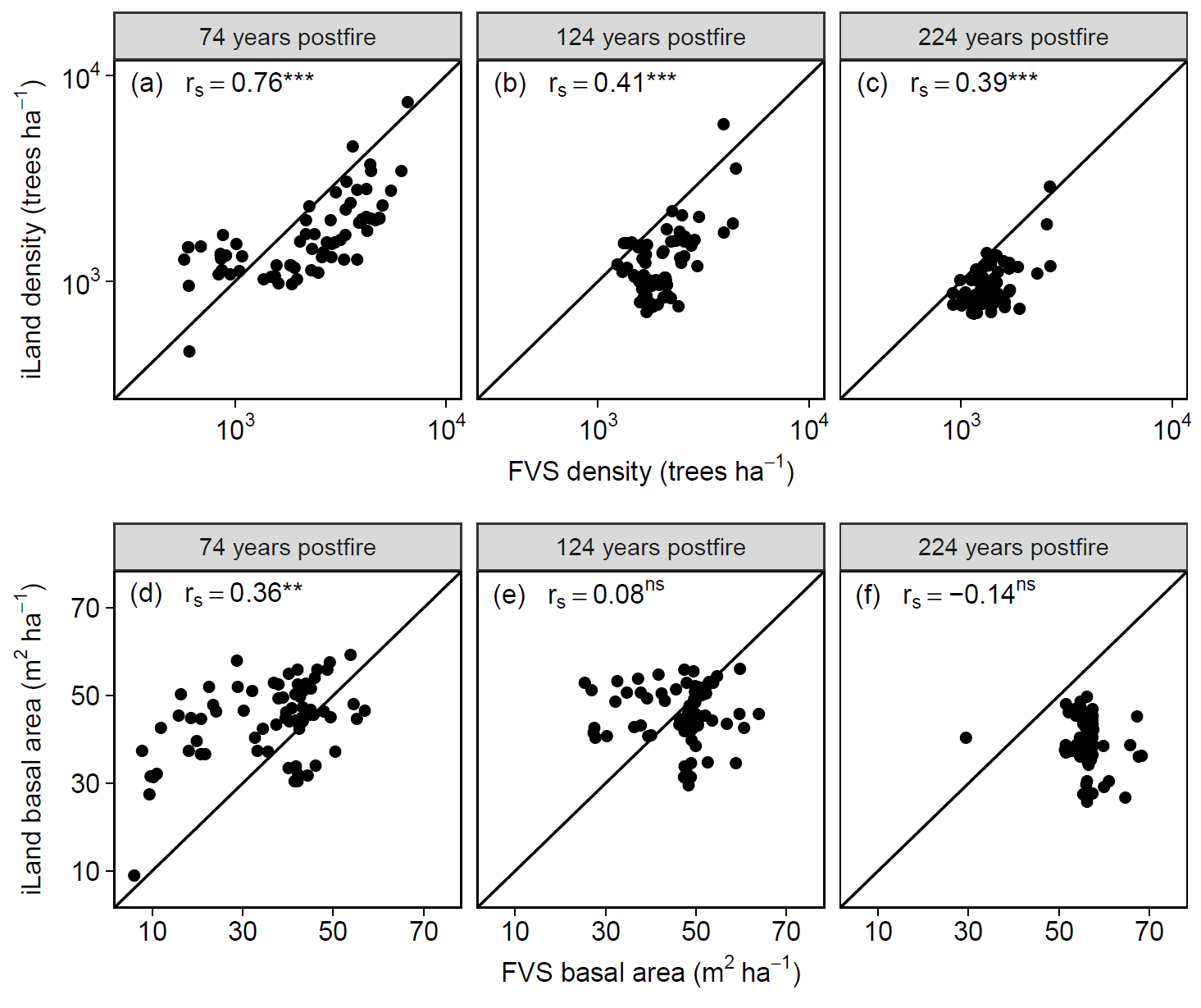
Productivity tests assess how well iLand characterizes structural trajectories and variability, e.g., tree densities, basal areas, and mean heights (Braziunas et al. 2018); basal area increment (Kobayashi et al. 2023); site index (Seidl, Rammer, et al. 2012); or dominant tree heights (Thom et al. 2022). The data available for comparison - e.g., yield tables (Albrich et al. 2018), Forest Inventory Data or independent field observations (Braziunas et al. 2018) - should be considered during the simulation setup. Most commonly monospecific stands are simulated under climate conditions representing the comparison data’s climate period and without additional disturbances. If the comparison data was measured in managed stands these management interventions should be mimicked in the simulations (Albrich et al. 2018). The simulation length varies depending on the comparison data (e.g., stand age, inventory frequency, etc.). If single-tree data is available from inventory plots, observed and predicted annual growth rates can also be compared. Success is gauged based on how well ranges or values of simulated data fit with the observed data and whether natural dynamics of stand development are reproduced (e.g., self-thinning).
Suggested setup
Use field observations and/or spatial iLand inputs to generate a set of stands that cover a low to high productivity gradient for the species of interest (i.e., an environmental gradient of less favorable to more favorable site conditions in which that species occurs).
Initialize trees in monospecific stands along this gradient and simulate stand development without allowing for interactions between stands (i.e., torus mode enabled).
Initial tree densities and sizes can be assigned based on field data or approximated using available data on stocking levels, stand density index, or stem density from yield tables for a given species.
Depending on the comparison data used, implement management prescriptions to control for stand density (e.g., when comparing to yield tables).
Do not simulate any disturbances.
Productivity experiments can be run with mortality and regeneration off, or with one or both turned on, at different stages of the process to focus on calibration or evaluation of different processes.
This same initial set of stands can typically be used for all subsequent stand-scale evaluations, including both monospecific and multispecies runs.
Calibration recommendations
For productivity experiments, tweak species parameters to better match comparison data. Remember, these are not expected to match perfectly and over-calibration of species to match one specific data set should be avoided. Review Seidl, Rammer, et al. (2012), Supplementary material for ideas of parameters to which productivity is most sensitive, and keep in mind which parameters are most uncertain versus ones that are fairly well defined. Here are some examples:
Simulated site index (SI) and diameter at breast height (DBH) are especially sensitive to: Response to plant-available nitrogen (
respNitrogenClass), minimum and optimum growth temperature (respTempMinandrespTempMax), shade tolerance (lightResponseClass), and height to diameter ratio (HDlowandHDhigh).Simulated SI and DBH are also sensitive to many biomass allometrics (
bmWoody,bmBranch, etc.), wood density, and form factor. These are generally well established parameters based on the literature or fit to empirical data, so avoid changing them unless nothing else works.Other parameters to consider tweaking, which are somewhere in between uncertain and well defined: Specific leaf area (
specificLeafArea, SLA, highly variable in the literature) and soil water response (psiMin, although note per the Seidl, Rammer, et al. (2012) sensitivity analysis, growth is not especially sensitive to this parameter).There are also some default, landscape, or biome-specific parameters or inputs to consider, but only if you have a consistent problem with productivity across all species. For example, potential light use efficiency (epsilon) has been adjusted in iLand applications in different regions. Another key driver of productivity is the environmental input data (e.g., soil fertility). If all stands are consistently underperforming, consider adjusting these values (e.g., bump up soil fertility across all stands/region).
Note that iLand also has an extensive set of debug outputs that you can turn on or off to help determine what is limiting tree growth or survival. For example,
Daily responseshelps you determine which factors among temperature, soil water availability, and vapor pressure deficit are most limiting growth for a given species at a daily time step. If you turn on daily responses, only run simulations for 1 or a few years, as these outputs can be quite large in size.
The aging (i.e., the decline in production efficiency with age) parameter must be iteratively calibrated. Mortality should be turned on, and stands should not be managed or subject to disturbance during aging calibration. Simulations should be run for longer than the maximum age of a given species. Then, iteratively adjust the coefficients of the aging equation so that:
Productivity declines with age, meaning that DBH and height curves are initially steep but shallow/flatten over time. Early seral species should be expected to have a more drastic decline in carbon use efficiency than late seral species.
Trees die as they approach max age and do not greatly overshoot max age.
Trees achieve reasonable maximum height and DBH. Keep in mind that maximum age, height, and DBH are theoretical maximum values. Whether and how close simulated trees are to these values should be based on your ecologically- and regionally-informed expectations.
For mortality experiments (after calibrating aging, keep motality on), consider the following:
If trees are dying too young or too quickly, consider adjusting
probIntrinsicorprobStress.If it seems like early mortality is due to low productivity and resulting carbon starvation, consider adjusting growth-related parameters described above. The debug outputs can help with this assessment, especially
Daily responses(e.g., if this output indicates a strong limitation of soil water, consider adjustingpsiMin).
Finally, the sapReferenceRatio parameter must also be iteratively calibrated. This can be done with the same set of stands (i.e., stands covering a wide environmental and productivity gradient where you expect to find the focal species). To do this make sure the species parameter sapReferenceRatio is set to 1 and regeneration is turned on in the project file. Then, start simulations from bare ground (no trees, saplings, or seedlings) with external seeds turned on for the species of interest and the establishment debug output (64) turned on. Run for a few years (e.g., 5-10 years). Update the species parameter sapReferenceRatio to the highest value for fEnvYr from the debug output.
Evaluation strategy
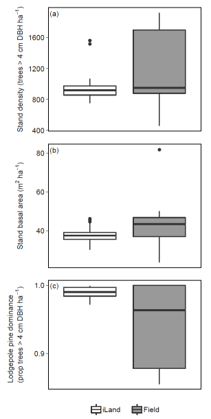
Depending on the evaluation, compare iLand simulations over time (e.g., how well do simulations overlap with comparison data) or at a specific point in time (e.g., year 100) with field observations or other empirically derived data (e.g., site index or yield estimates for year 100). “Over time” comparisons evaluate how well simulations cover the range of comparison data, qualitatively and quantitatively. “Point in time” comparisons evaluate how well simulations correspond with comparison data via scatterplots, boxplots, and 1:1 lines. Model performance can be evaluated using quantitative comparisons such as root mean squared error (RMSE), slope, bias, correlation (r), goodness of fit (R2), or other metrics.
Mortality evaluations can also include comparisons with general empirical self-thinning coefficients (Seidl, Rammer, et al. 2012).
10.2 PNV, regeneration, and competition
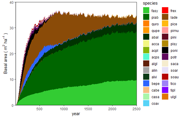
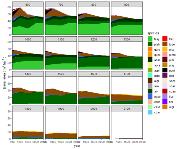
Potential natural vegetation (PNV) evaluations assess how well iLand characterizes successional trajectories and species composition in late-seral stages. This can be done at stand or landscape scales. Field observations for a given forest type (Braziunas et al. 2018), inventory data (Kobayashi et al. 2023), or descriptive accounts of the potential natural vegetation (Albrich et al. 2018; Thom et al. 2022) can be used for comparison. Simulations are usually started from bare ground with external seeds supplied (e.g., via seed belts) and run for 100s-1000s of years under historical climate conditions with no management. Longer time periods are necessary for landscape PNVs, because species will usually only enter from the edges of landscape. PNV simulations can be configured to include or exclude disturbances. For example, disturbances may be excluded from stand-scale PNVs to view stand development and successional trajectories. Or, for landscapes where forest structure and species composition is strongly shaped by disturbances, PNV simulations should consider including the relevant disturbance regimes so that outcomes will better align with expectations. Success is gauged based on how well iLand reproduces typical successional patterns and anticipated species composition (e.g., stratified by forest types or elevation zones).
Suggested setup
For stand-scale evaluations:
Stands should be selected based on having environmental conditions that are representative for a given dominant species, forest type, or species mix. These could be all or a subset of stands used for productivity evaluations described above. Alternatively, stands could be selected by using other spatial data (e.g., a forest type map, an elevational gradient) to identify representative locations within a study region or iLand landscape.
Initialize stands either with seedlings or starting from bare ground. When starting from bare ground, seeds can come from a surrounding seed belt with user-defined species composition (e.g., approximated or field-derived composition for the given forest type or specific stand) to simulate post-disturbance or -clearing successional trajectories. Alternatively, bare ground simulations can be run with equal, very low probability of seed inputs for all potentially present species and run for 100s to 1000s of years to simulate equilibrium species composition and dominance for a given set of environmental conditions.
Landscape-scale setups require compiling landscape extent, biophysical drivers, and vegetation conditions as described in the Setting up landscapes chapter. It is also important to consider disturbances at this stage, because the PNV for a landscape may be strongly shaped by past disturbances. These could be natural disturbances such as bark beetle outbreaks or fire, or disturbances due to human management. The PNV should be run starting from bare ground, meaning no trees, saplings, or seedlings on the landscape.
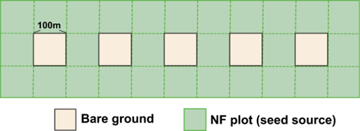
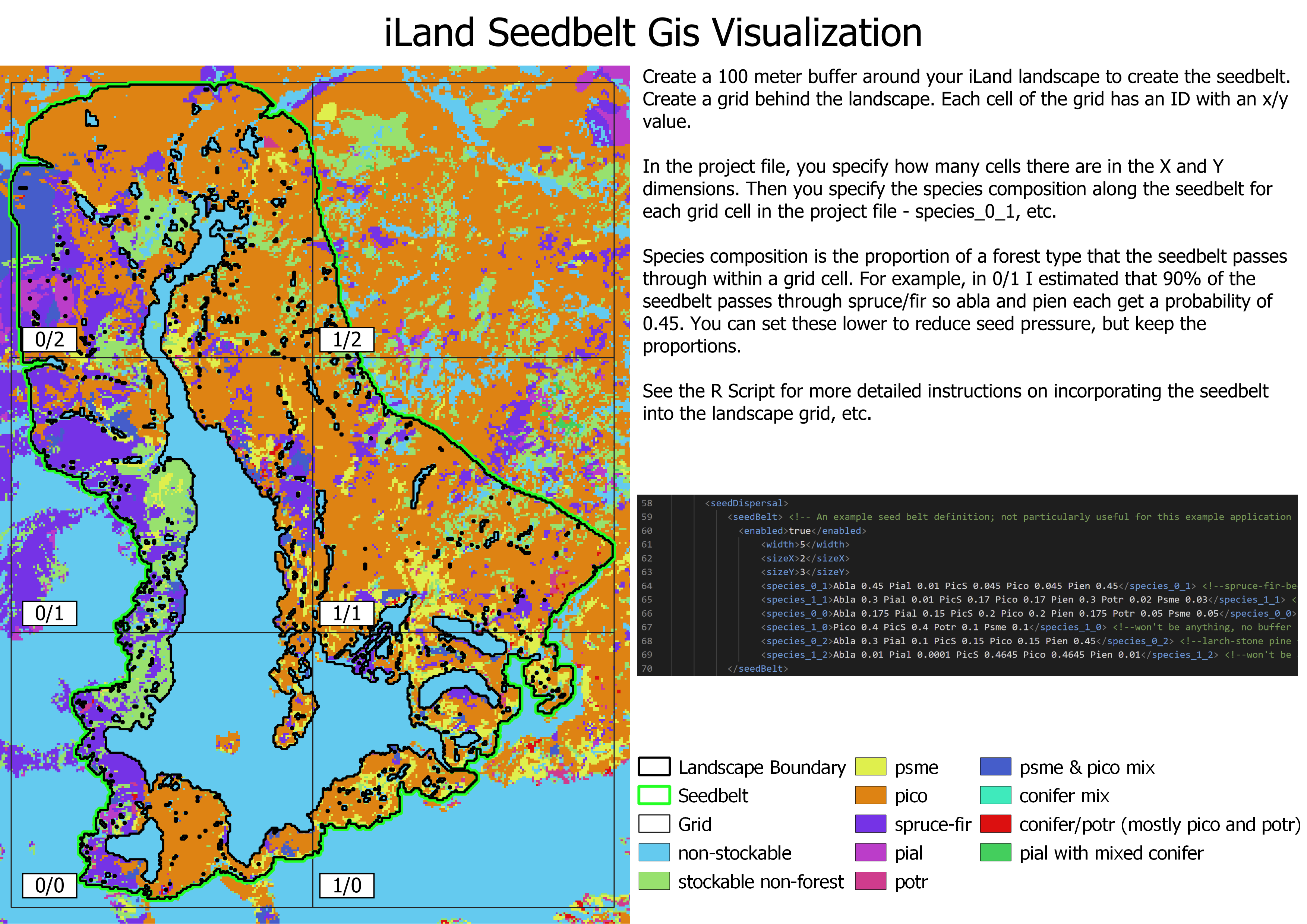
The first step is to create a seed belt (see Figure 10.1) around the edge of the landscape that represents the surrounding forest. See the iLand wiki external seeds page for more information. The seed belt should be adjacent to the forested edges of the landscape and should take topography and other landscape features into consideration (e.g., you might expect seeds to enter from the bottom of a valley but not from the top of a mountain, you would not expect seeds to arrive from a lake). The species composition of the seed belt should take into consideration the forest type that you expect to be there, or that is present today, but it is essential that seeds from all species present in the landscape are present in at least some proportion. Otherwise, they will never be able to migrate in.
The landscape PNV should then be run under historical climate for enough years for species to migrate into the landscape and achieve some sort of equilibrium relative to the drivers (which would include climate, soils, and disturbances). This is usually at least 1000 years, but can often be longer (e.g., 2500 years for Berchtesgaden examples included above). If there is a lot of variability, such as in disturbance regimes, PNVs can be run for multiple replicates or the results from the last ~100 years or so can be averaged.
Calibration recommendations
First, the sapReferenceRatio parameter must be iteratively calibrated (see the comment above on this topic).
The stand-scale setup is well suited for calibrating multiple species parameters. A suggested progression is to first simulate monospecific stands with initial seedlings or external seeds to calibrate species-specific sapling survival and growth. When running these simulations, ask:
Are saplings surviving? If not, consider adjusting survival-related parameters (
sapMaxStress,SapStressThreshold).Are seedlings establishing? If not, consider adjusting establishment-related parameters. Look at the establishment debug output to get a sense of what factors might be most limiting. Note that some parameters set thresholds that give a yes/no for establishment, whereas others control establishment probability. For more information, see the iLand wiki.
Are forested conditions being maintained over time and generally covering the range of expected densities and structures? Use the run with no external seed input to focus on whether seed supply and forested conditions are being maintained over time. If subsequent generations after the initial cohorts are not maintaining the forest, consider parameters associated with seed supply (
maturityYears,seedYearInterval,nonSeedYearFraction,fecundity). If stand densities and structures are low, consider adjustingsapReinekesR, which determines how many trees will be recruited as individuals when sapling cohorts pass the 4 m threshold. Do not spend too much time worrying about the sapling densities themselves, as these rely on this same multiplier. It is more important and ecologically meaningful for the model to get the tree densities right.Are saplings growing fast enough? If not, consider adjusting
sapHeightGrowthPotential. However, this is usually parameterized with with empirical data, so it generally should align with expectations. Comparison data on sapling age versus height can help facilitate the calibration of this parameter.
Next, use stand-scale simulations starting from bare ground, with seeds available from multiple species via either the seed belt or external seed, to calibrate parameters that influence interspecific competition and relative dominance. Parameters to focus on calibrating include:
Regeneration parameters, especially
sapReinekesR,fecundity, and other seed supply parameters (maturityYears,seedYearInterval,nonSeedYearFraction,fecundity).Seedling establishment parameters (see establishment and species parameter wiki pages) if a given species is not establishing, or sapling growth/mortality parameters (
sapHeightGrowthPotential,sapMaxStress,SapStressThreshold) if establishment is occurring but the species is not “winning” the race to become a tree.If saplings are being recruited but trees are not competitive, consider parameters that may affect relative tree growth along environmental gradient such as response to plant-available nitrogen (
respNitrogenClass), minimum and optimum growth temperature (respTempMinandrespTempMax), shade tolerance (lightResponseClass), and soil water response (psiMin). You could also consider some of the mortality parameters, such asprobIntrinsicandprobStress. Whenever making changes to any of these, rerun the productivity and mortality experiments from above to check that they still correspond well.
Evaluation strategy
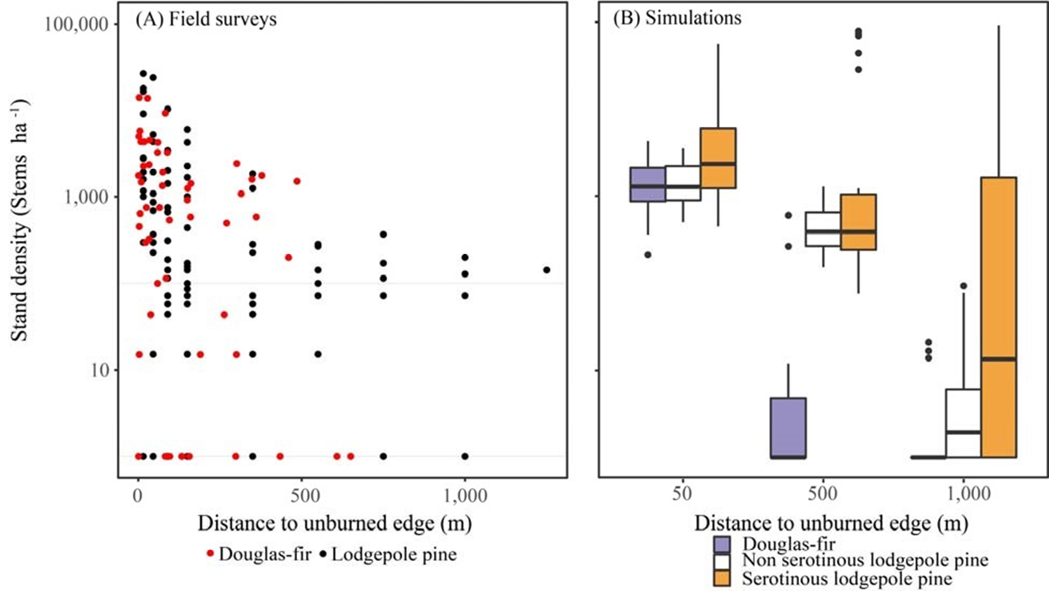
Stand-scale regeneration simulations can be used to evaluate single-species behavior if comparison data is available, such as sapling growth over time or seedling establishment relative to distance from seed source (Hansen et al. 2018).
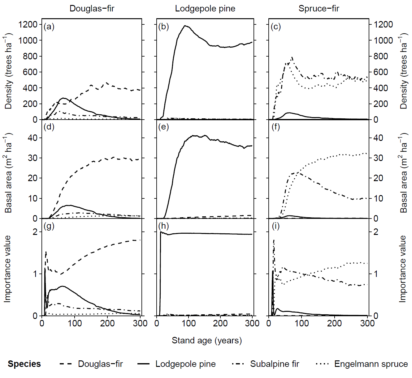
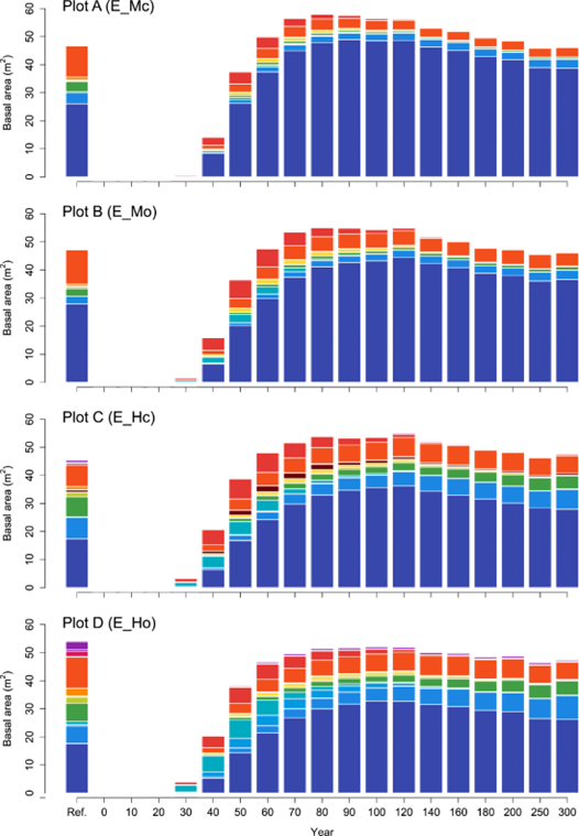
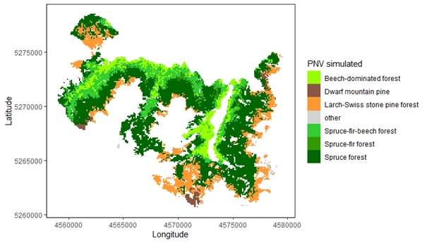
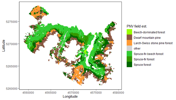
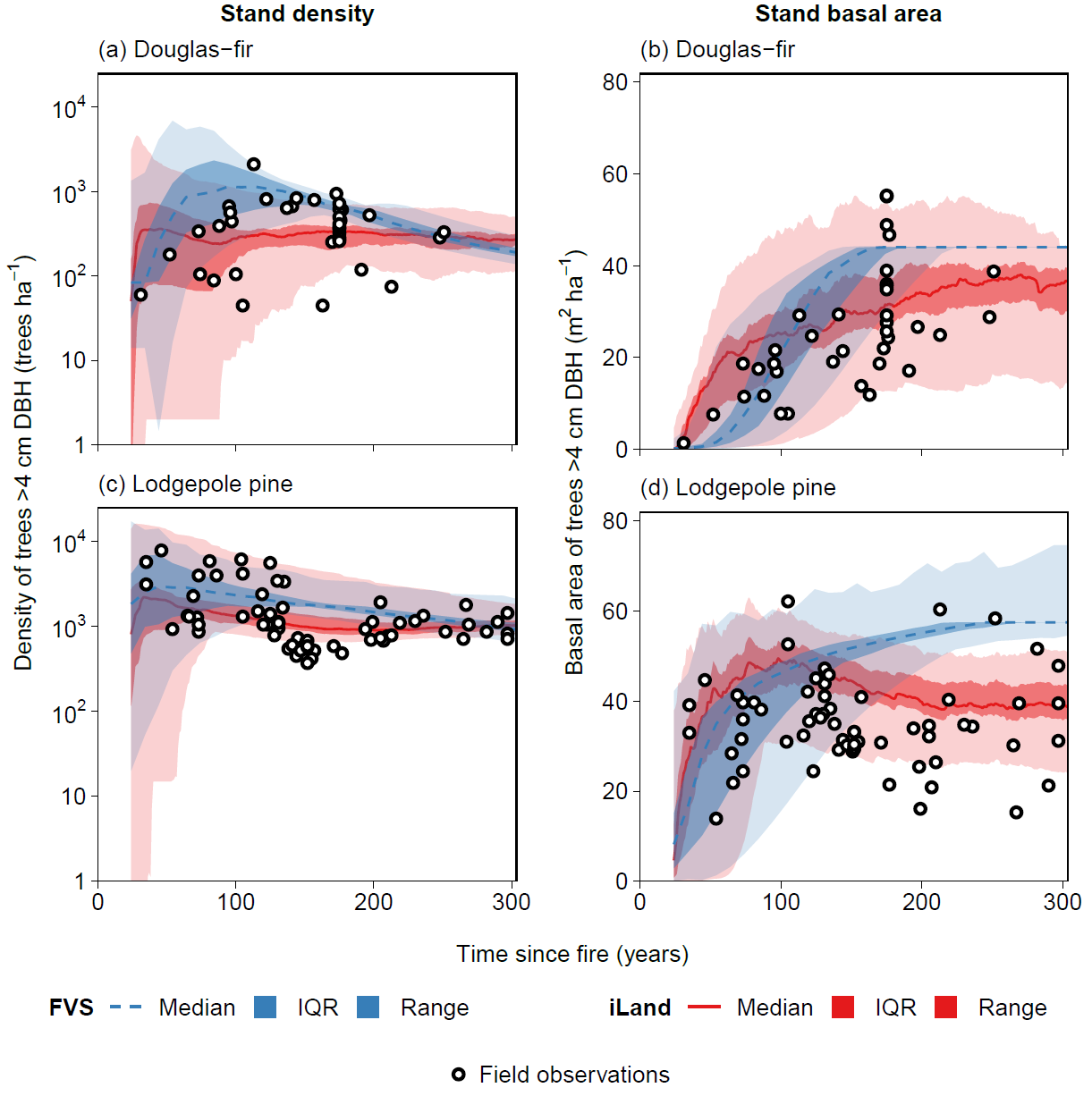
Multispecies evaluations can include quantitative comparisons (e.g., goodness of fit), qualitative checks for general consistency with the distribution of field observations (e.g., comparison with stand density, basal area, and importance value over time or at specific stand ages; comparison of relative basal area shares by species over time with field observations), and/or expert assessment based on ecological expectations (e.g., evaluation of equilibrium or PNV simulations along a forest type or elevational gradient). At the end of a PNV simulation, a simulated forest type map can be created for comparison with a map of current forest types or with expectations (e.g., if management history has altered current forest types from their expected PNV conditions).
10.3 Other evaluation tests
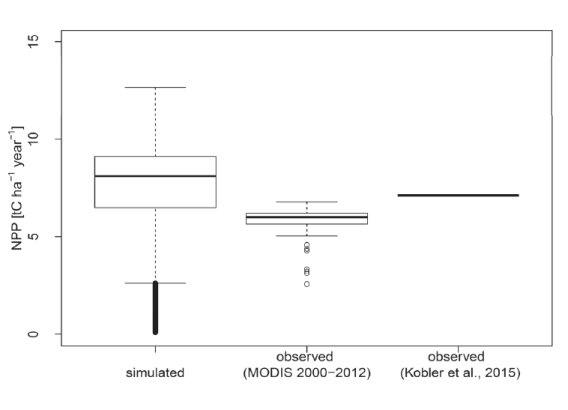
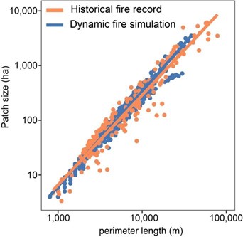
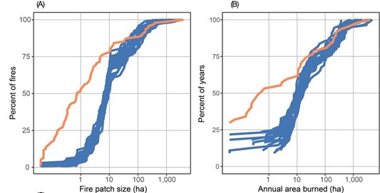
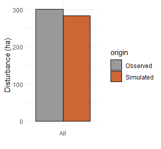
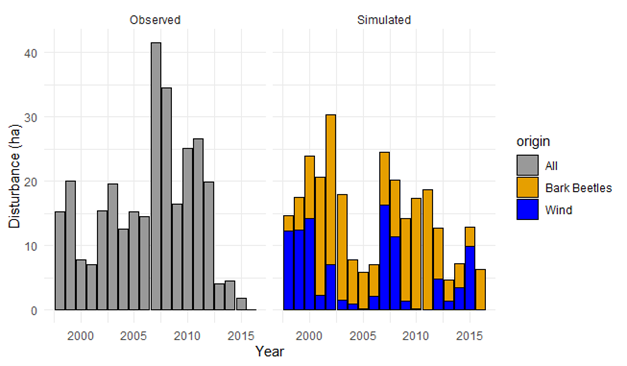
Other possible evaluation tests include comparisons with other models (Braziunas et al. 2018); equilibrium simulations (Albrich, Rammer, and Seidl 2020); and tests of specific modules such as management (Albrich et al. 2018), disturbances (e.g., comparison against remote sensing products) (Hansen et al. 2020; Thom et al. 2022), or carbon and nitrogen cycling (Seidl, Spies, et al. 2012; Albrich et al. 2018; Hansen et al. 2020).
10.4 Concluding thoughts: Making parameters robust and adaptable through ongoing evaluation
Parameterized and calibrated species must strike a balance between accuracy within a specific region and generality to replicate patterns across diverse environments. As a goal, you want to be able to use the same species parameters across a wide range of environmental conditions, in new landscapes, and throughout a region or biome. You should re-evaluate whether species are behaving as expected every time you apply them in a new area or if you are adding new species to the pool. A useful approach is to create an automated pipeline allowing you to re-run the evaluations referenced above for your existing and new species pools, using the same set of stands and landscapes used in initial calibrations. This will allow you to identify effects of new changes on species behavior and interactions. By continuing to add evaluations for new regions and new landscapes, this should also make the species parameter sets more robust and reliable over time and across broader extents. It can also help identify when regional variants for species species, or entire species sets, are necessary. For example, the iLand team has developed the “Permanent Evaluation and Testing Suite” (PETS) framework for Central European tree species, which enables standardized evaluation of changes in species parameters for all simulated forests with available data for model evaluation.