5 iLand outputs
iLand can provide a wealth of output data, with differing spatial and temporal resolution and on different levels of aggregation. The standard way is via “outputs”, which are described now. Outputs in iLand are per default created as a SQLite database. Every type of output is represented by one table within this output database, and the user controls which outputs are active. Thus, the results of one simulation run are contained in one single file. Each iLand output database contains a small table named runinfo which stores a timestamp when the simulation was started, and iLand version information.
Since iLand is a dynamic simulation model, most outputs have a time-dimension; many outputs describe stocks (at a certain point in time) or flows (for a specific period). Data can be very fine-grained - for example, the tree output contains a single row for every tree and for every year of the simulation. This is not practical (particularly on landscape scale!), therefore different levels of aggregation are possible. For example, the landscape output describes average values for timber volume, biomass, etc. for each species but for the whole landscape. While you (technically) can enable all outputs all the time, it is usually not practical to do so. With more outputs enabled, simulation results take up moch more disk space. In addition, the time for running the simulation (more data to wrote) but also the time for analyzing the data (more data to process!) goes up. Striking the right balance here is particularly important for large simulation jobs with hundreds of individual simulation runs.
5.1 Output database
The output database is written to a location specified in the project file. Basically, there are two options:
reuse a database file: in this case every run will overwrite the preceding run. This is an option when still “playing around”.
create a database for each run: this is clearly the option of choice for larger simulation jobs.
The filename of the output-database is defined by the home.database.out key in the project file. If this key contains a simple string, a database with that is opened (and overwritten). If you want to go with option 2, a special syntax can be used for the filename to automatically add a time (unique) timestamp. To do this, add $ ch (e.g. projectX_$date$.db), where the string between the $date$-signs is replaced with a time stamp value (e.g. “20091021_143059”).
5.2 Controlling outputs
The iLand wiki contains a list with the detailed definition of all available outputs under https://iland-model.org/outputs. Currently, iLand provides ~25 different “outputs”. Each output is configured by a corresponding section in the project file (in the section output). Every output can be turned on or off (using the enabled key), and some can be further customized, in many cases to limit the generation of output data, e.g. by limiting an output to only run every 10 years.
Here is an example in the XML project file:
 <output>
    <tree> <!-- individual tree output -->
      <enabled>tree</enabled>
      <filter>year=10 or year=20</filter>
    </tree>
    <treeremoved> <!-- individual tree output -->
      <enabled>false</enabled>
      <filter></filter>
    </treeremoved>
    ....
In this example, the output tree is turned on, but writes data only in year 10 or 20. The output treeremoved is disabled.
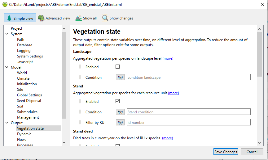
The Settings editor provides a graphical user interface for configuring (most) aspects of outputs, see Figure 5.1.
5.3 Other types of outputs
In addition to the standard “outputs” described above, iLand provides more ways to extract / store data.
One option are “debug outputs” (https://iland-model.org/Debug+Outputs): Debug outputs are more low-level and typically highly detailed outputs. While not very useful for standard applications, there are cases where the high level of details may be important. For example, debug output allow to to track changes in the water cycle with daily resolution. Debug outputs are in the form of simple CSV text files and have some quirks (e.g. the way how to enable / disable them)
Another option is gridded data: here you use JavaScript to access spatial data in iLand and write to raster files. This can be rather straightforward (write a map of basal area for a given species every 10 years), but can involve relatively complex (spatial) computation. Below is (a rather complex) example. See Scripting chapter and https://iland-model.org/apidoc/classes/Grid.html for more details!
var wind_grid; // global variable to hold the grid

// this event / function is called by the wind disturbance module
// the function keeps a running sum for each 10m pixel and
// counts the trees that were killed on a cell
function onAfterWind() {
   if (wind_grid == undefined)
       wind_grid = Wind.grid("treesKilled");

   var g = Wind.grid("treesKilled"); // killed this year
   // add to the total number of trees killed:
   wind_grid.combine( 'killed_sum +
   killed_now', { killed_sum: wind_grid, killed_now: g } );
}

// this function is called by iLand at the end of every simulation year
function onYearEnd() {
    if (Globals.year % 20 == 0) {
      // every 20 years run a spatial analysis to find contiguous patches
// (of cells that were affected by wind in the last 20 yrs)
        var p = wind_grid = SpatialAnalysis.patches(wind_grid, 5);
        Globals.saveTextFile(Globals.defaultDirectory('output') +
        '_stormPatches_' + Globals.year + '.txt',
        SpatialAnalysis.patchsizes + "\n");
        wind_grid = Wind.grid("treesKilled"); // +- reset the variable
    }
}
5.4 Analyzing iLand outputs
Once iLand has finished a simulation, you can start to look at the results of the simulation. In most cases this process requires to analyse the content of the output database (see above). A typical approach (many different approaches exist!) is to use R to do the job. The basic pattern could look like this:
open the data base in R. For this the
RSQLiteR package is very usefulread the tables (i.e., the “outputs”) of interest
do some data wrangling (e.g. using the
dplyrpackage)plot results
Here is a very simple example showing the approach:
library(RSQLite) # load the RSQLite package to work with SQLite databases

# Step 1 - load the data
# open the output data base of the simulation and read the "landscape" output.
# Adopt the file name!
db <- dbConnect(RSQLite::SQLite(), "output/output.sqlite")
lscp <- dbReadTable(db, "landscape")
dbDisconnect(db)
summary(lscp) ## show some stats

# Step 2 - analyse the data
library(ggplot2)
library(dplyr)
# plot time series of volume/ha for spruce and beech
ggplot(lscp %>% filter(species %in% c("piab", "fasy")),
       aes(year, volume_m3, col=species)) +
  geom_line()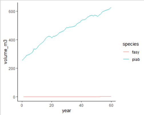
5.5 Data analysis with R - real world example
The following shows a real-world data analysis example with R and R markdown.
Christina Dollinger
April 16th, 2024
# # # # # # #
# Set-up ####
# # # # # # #

## Read in libraries ####
library(tidyverse, warn.conflicts = FALSE, verbose = FALSE)
## ── Attaching packages ─────────────────────────────────────── tidyverse 1.3.2 ──
## ✔ ggplot2 3.4.0 ✔ purrr 1.0.1
## ✔ tibble 3.2.1 ✔ dplyr 1.1.0
## ✔ tidyr 1.3.0 ✔ stringr 1.5.0
## ✔ readr 2.1.3 ✔ forcats 1.0.0
## ── Conflicts ────────────────────────────────────────── tidyverse_conflicts() ──
## ✖ dplyr::filter() masks stats::filter()
## ✖ dplyr::lag() masks stats::lag()library(RSQLite, warn.conflicts = FALSE)
library(dbplyr, warn.conflicts = FALSE)
library(terra, warn.conflicts = FALSE)## terra 1.7.3## Read in iLand input files ####
# Environment file
env.df <- read_delim("../gis/environment.txt"); head(env.df)## Rows: 13372 Columns: 20
## ── Column specification ────────────────────────────────────────────────────────
## Delimiter: " "
## chr (1): model.climate.tableName
## dbl (19): id, x, y, model.site.availableNitrogen, model.site.soilDepth, mode...
##
## ℹ Use `spec()` to retrieve the full column specification for this data.
## ℹ Specify the column types or set `show_col_types = FALSE` to quiet this message.## # A tibble: 6 × 20
## id x y model.…¹ model…² model…³ model…⁴ model…⁵ model…⁶ model…⁷
## <dbl> <dbl> <dbl> <chr> <dbl> <dbl> <dbl> <dbl> <dbl> <dbl>
## 1 1 4575958 5260680 climate4 40.3 5 44 35 21 9039.
## 2 2 4571758 5260680 climate1 39.8 11.7 50 32 18 7397.
## 3 3 4576258 5260780 climate… 44.1 20 44 35 21 480.
## 4 4 4575758 5260780 climate… 40.4 15 30 40 30 10850.
## 5 5 4571758 5260780 climate… 39.9 5 44 35 21 12466.
## 6 6 4571558 5260780 climate8 40.5 5 44 35 21 11134.
## # … with 10 more variables: model.site.youngLabileN <dbl>,
## # model.site.somC <dbl>, model.site.somN <dbl>,
## # model.site.youngRefractoryC <dbl>, model.site.somDecompRate <dbl>,
## # model.site.soilHumificationRate <dbl>,
## # model.initialization.snags.swdC <dbl>,
## # model.initialization.snags.swdCount <dbl>,
## # model.initialization.snags.swdHalfLife <dbl>, …# DEM raster, 50 x 50 m resolution
dem.grid <- rast("../gis/npbg_dem50fix.asc")
# Add information about elevation to environment file
env.df$elevation <- terra::extract(
# aggregate DEM to fit resolution of environment file
terra::aggregate(dem.grid, fact = 2, fun = "mean"),
env.df[, c("x", "y")], ID = FALSE) %>% unlist()
# Species database
db.conn <- dbConnect(RSQLite::SQLite(),
dbname = "../database/species_param_europe.sqlite")
species.df <- tbl(db.conn, "species") %>%
collect()
dbDisconnect(db.conn); rm(db.conn)
# # # # # # # # # # # # # #
# Read in iLand output ####
# # # # # # # # # # # # # #
db.conn <- dbConnect(RSQLite::SQLite(),
dbname = "../output/output.sqlite") # connect to output sqlite
RSQLite::dbListTables(db.conn) # list of available output tables## [1] "barkbeetle" "dynamicstand" "landscape" "runinfo" "wind"lscp <- tbl(db.conn, "landscape") %>%
collect()
dyn <- tbl(db.conn, "dynamicstand") %>%
filter(year %in% c(0,100)) %>% # filter simulation years
rename(id = rid) %>%
collect() %>%
# combine with environment file to get information like xy-coordinates or elevation for each Resource Unit
left_join(env.df[, c("id", "x", "y", "elevation")],
by = join_by(id))
wind <- tbl(db.conn, "wind") %>%
collect()
dbDisconnect(db.conn); rm(db.conn)
# # # # # # # #
# Analysis ####
# # # # # # # #
## a. Landscape output ####
most_common_species <- lscp %>% # most common species by basal area in year 0
filter(year == 0) %>%
arrange(desc(basal_area_m2)) %>%
slice(1:5) %>%
arrange(species) %>%
pull(species)
most_common_species_color <- species.df %>% # get display color used by iLand for the species
arrange(shortName) %>%
filter(shortName %in% most_common_species) %>%
mutate(displayColor = paste0("#", displayColor)) %>%
pull(displayColor) %>%
c("#808080") # color for "other" species
names(most_common_species_color) <- c(most_common_species, "other")
summary(lscp)## year area area_100m species
## Min. : 0.00 Min. :1718 Min. :2272 Length:2793
## 1st Qu.: 26.00 1st Qu.:1718 1st Qu.:2272 Class :character
## Median : 51.00 Median :1718 Median :2272 Mode :character
## Mean : 50.48 Mean :1718 Mean :2272
## 3rd Qu.: 76.00 3rd Qu.:1718 3rd Qu.:2272
## Max. :100.00 Max. :1718 Max. :2272
## count_ha dbh_avg_cm height_avg_m volume_m3
## Min. : 0.0000 Min. : 0.000 Min. : 0.000 Min. : 0.00000
## 1st Qu.: 0.0047 1st Qu.: 3.486 1st Qu.: 4.272 1st Qu.: 0.00002
## Median : 0.6882 Median : 5.103 Median : 5.177 Median : 0.00342
## Mean : 34.4830 Mean : 6.338 Mean : 5.481 Mean : 10.70062
## 3rd Qu.: 6.5219 3rd Qu.: 6.742 3rd Qu.: 6.497 3rd Qu.: 0.09341
## Max. :509.8848 Max. :41.453 Max. :21.442 Max. :268.95025
## total_carbon_kg gwl_m3 basal_area_m2 NPP_kg
## Min. : 0.00 Min. : 0.0000 Min. : 0.000000 Min. : 0.000
## 1st Qu.: 0.04 1st Qu.: 0.0001 1st Qu.: 0.000006 1st Qu.: 0.004
## Median : 6.35 Median : 0.0364 Median : 0.001154 Median : 0.551
## Mean : 4189.97 Mean : 17.9192 Mean : 1.085451 Mean : 525.470
## 3rd Qu.: 105.37 3rd Qu.: 0.3967 3rd Qu.: 0.034707 3rd Qu.: 18.750
## Max. :96908.96 Max. :564.9400 Max. :25.058179 Max. :12836.768
## NPPabove_kg LAI cohort_count_ha
## Min. : 0.000 Min. :0.0000000 Min. : 0.00
## 1st Qu.: 0.002 1st Qu.:0.0000012 1st Qu.: 0.00
## Median : 0.307 Median :0.0001775 Median : 4.00
## Mean : 314.496 Mean :0.1232238 Mean : 50.02
## 3rd Qu.: 10.847 3rd Qu.:0.0042951 3rd Qu.: 42.00
## Max. :7874.235 Max. :3.0285868 Max. :441.00# Bar plot showing basal area development by species over the 100-year simulation period
lscp %>%
mutate(species_new = ifelse(species %in% most_common_species, species, "other")) %>%
ggplot(aes(x = year, y = basal_area_m2, fill = species_new)) +
geom_bar(stat = "identity") +
scale_fill_manual(values = most_common_species_color) +
labs(x = "Simulation year", y = "Mean basal area [m²/ha]", fill = "Species code",
title = "Basal area development by species over the 100-year simulation period") +
theme_bw()

## b. Dynamic stand output ####
summary(dyn)
## year ru id species
## Min. : 0.00 Min. : 0 Min. : 4713 Length:25679
## 1st Qu.: 0.00 1st Qu.: 708 1st Qu.: 7545 Class :character
## Median :100.00 Median :1242 Median : 9333 Mode :character
## Mean : 59.04 Mean :1201 Mean : 9196
## 3rd Qu.:100.00 3rd Qu.:1717 3rd Qu.:10934
## Max. :100.00 Max. :2271 Max. :12564
## dbh_mean dbh_sd dbh_p5 dbh_p95
## Min. : 2.351 Min. : 0.0000 Min. : 2.325 Min. : 2.351
## 1st Qu.: 5.555 1st Qu.: 0.2682 1st Qu.: 3.870 1st Qu.: 6.003
## Median :11.485 Median : 3.3833 Median : 5.038 Median :21.418
## Mean :17.383 Mean : 5.0077 Mean :11.102 Mean :25.659
## 3rd Qu.:27.526 3rd Qu.: 8.3080 3rd Qu.:14.729 3rd Qu.:42.857
## Max. :83.175 Max. :35.9481 Max. :83.175 Max. :99.347
## height_mean height_sd age_mean age_sd
## Min. : 1.893 Min. : 0.0000 Min. : 6.50 Min. : 0.000
## 1st Qu.: 4.589 1st Qu.: 0.2453 1st Qu.: 35.75 1st Qu.: 0.000
## Median : 9.537 Median : 2.1001 Median : 67.05 Median : 5.852
## Mean :11.523 Mean : 2.9363 Mean : 90.39 Mean : 18.233
## 3rd Qu.:17.324 3rd Qu.: 4.9807 3rd Qu.:131.08 3rd Qu.: 29.162
## Max. :41.068 Max. :16.3171 Max. :437.00 Max. :169.000
## if_height_5_1_0_sum if_height_5_and_height_10_1_0_sum
## Min. : 0.00 Min. : 0.00
## 1st Qu.: 0.00 1st Qu.: 0.00
## Median : 2.00 Median : 1.00
## Mean : 15.14 Mean : 26.08
## 3rd Qu.: 11.00 3rd Qu.: 15.00
## Max. :1362.00 Max. :1379.00
## if_height_10_and_height_15_1_0_sum if_height_15_and_height_20_1_0_sum
## Min. : 0.00 Min. : 0.0
## 1st Qu.: 0.00 1st Qu.: 0.0
## Median : 0.00 Median : 0.0
## Mean : 18.65 Mean : 16.4
## 3rd Qu.: 12.00 3rd Qu.: 8.0
## Max. :787.00 Max. :592.0
## if_height_20_and_height_25_1_0_sum if_height_25_and_height_30_1_0_sum
## Min. : 0.00 Min. : 0.000
## 1st Qu.: 0.00 1st Qu.: 0.000
## Median : 0.00 Median : 0.000
## Mean : 12.96 Mean : 6.855
## 3rd Qu.: 4.00 3rd Qu.: 2.000
## Max. :615.00 Max. :253.000
## if_height_30_and_height_35_1_0_sum if_height_35_and_height_40_1_0_sum
## Min. : 0.000 Min. : 0.0000
## 1st Qu.: 0.000 1st Qu.: 0.0000
## Median : 0.000 Median : 0.0000
## Mean : 2.569 Mean : 0.6864
## 3rd Qu.: 0.000 3rd Qu.: 0.0000
## Max. :269.000 Max. :108.0000
## if_height_40_and_height_45_1_0_sum if_height_45_and_height_50_1_0_sum
## Min. : 0.00000 Min. :0.0000000
## 1st Qu.: 0.00000 1st Qu.:0.0000000
## Median : 0.00000 Median :0.0000000
## Mean : 0.05382 Mean :0.0009736
## 3rd Qu.: 0.00000 3rd Qu.:0.0000000
## Max. :58.00000 Max. :2.0000000
## if_height_50_1_0_sum x y elevation
## Min. :0.0000000 Min. :4559058 Min. :5267880 Min. : 789.3
## 1st Qu.:0.0000000 1st Qu.:4560958 1st Qu.:5270480 1st Qu.: 960.0
## Median :0.0000000 Median :4561958 Median :5271680 Median :1163.6
## Mean :0.0008567 Mean :4561955 Mean :5271640 Mean :1204.8
## 3rd Qu.:0.0000000 3rd Qu.:4562958 3rd Qu.:5272880 3rd Qu.:1400.9
## Max. :3.0000000 Max. :4564458 Max. :5274980 Max. :2004.4# Map showing mean DBH of Picea abies in simulation year 0 versus year 100
dyn %>%
filter(species == "piab") %>%
ggplot(aes(x = x, y = y, fill = dbh_mean)) +
geom_tile() +
facet_wrap(~year) +
coord_equal() +
scale_fill_distiller(palette = "PuRd", direction = 1) +
labs(fill = "Mean DBH [cm]",
title = "Mean DBH of Picea abies in simulation year 0 (left) versus year 100 (right)") +
theme_bw()

# Line plot showing relationship between elevation and mean DBH by species
dyn %>%
  filter(year == 100,
         species %in% c("piab", "lade", "pice")) %>%
  dplyr::select(year, id, x, y, species, dbh_mean, elevation) %>%
  mutate(elevation_rounded = round(elevation/10)*10) %>%
  group_by(species, elevation_rounded) %>%
  summarise(dbh_mean_elevation = mean(dbh_mean),
            dbh_sd_elevation = sd(dbh_mean)) %>%
  ggplot(aes(x = elevation_rounded, y = dbh_mean_elevation, col = species,
             ymin = dbh_mean_elevation - dbh_sd_elevation,
             ymax = dbh_mean_elevation + dbh_sd_elevation, fill = species)) +
  geom_ribbon(alpha = 0.6) +
  geom_line(linewidth = 2, col="black") +
  geom_line(linewidth = 1) +
  scale_fill_manual(values = most_common_species_color) +
  scale_color_manual(values = most_common_species_color) +
  labs(x = "Elevation (in 10 m steps)", y = "Mean DBH per elevation step [cm]", fill = "Species code",
       col = "Species code", title = "Relationship between elevation and mean DBH by species\nSimulation year 100; ribbon showing mean +/- sd") +
  theme_bw()

## c. Wind output ####
summary(wind)
## year iterations windspeed_ms direction area_ha
## Min. : 1.00 Min. :73 Min. :11.55 Min. : 58.0 Min. : 0.440
## 1st Qu.:15.00 1st Qu.:73 1st Qu.:11.66 1st Qu.:252.0 1st Qu.: 1.110
## Median :32.00 Median :73 Median :12.08 Median :277.0 Median : 2.490
## Mean :45.83 Mean :73 Mean :12.35 Mean :263.6 Mean : 6.957
## 3rd Qu.:79.00 3rd Qu.:73 3rd Qu.:12.56 3rd Qu.:299.0 3rd Qu.: 5.050
## Max. :99.00 Max. :73 Max. :16.76 Max. :345.0 Max. :86.140
## killedTrees killedBasalArea killedVolume
## Min. : 127 Min. : 7.487 Min. : 87.82
## 1st Qu.: 718 1st Qu.: 35.469 1st Qu.: 417.84
## Median : 1776 Median : 101.754 Median : 1232.51
## Mean : 4489 Mean : 231.270 Mean : 2503.04
## 3rd Qu.: 2790 3rd Qu.: 158.693 3rd Qu.: 1771.60
## Max. :62098 Max. :3093.925 Max. :32739.85# Line plot showing basal area killed over the 100-year simulation period
wind %>%
ggplot(aes(x = year, y = killedBasalArea)) +
geom_line() +
labs(x = "Simulation year", y = "Basal area killed by wind [m²/ha]",
title = "Wind disturbances: basal area killed over the 100-year simulation period") +
theme_bw()
