Table of contents
Background
The initialization of vegetation and soil properties in iLand has always been a rather complicated and labor intensive task. The process typically included the combination of different data sources with different spatial and temporal scales; missing attributes required often rough estimates (e.g., regeneration, belowground carbon pools) or other workarounds. The end product of this process was the initialization of the current state of the forest (e.g., dbh and height distributions of small homogeneous stands), which typically reflected the available data as closely as possible, but was still to some degree “synthetic” (e.g., because of inventory datasets and remote sensing datasets were recorded for different points in time). An example for this approach to initialize iLand is described in detail in Thom et al. (2016).
The main problem with this approach (in addition to the large amount of work): the synthetic vegetation state is not necessarily compatible with the internal logic of the model. For example, individual trees may get assigned to positions which do not receive enough light for a sustained existence – as a consequence such trees die early in a simulation. Another example is the vertical stand structure where the “synthetic” structure can deviate substantially from a “grown” structure. This can be a problem with the simulation of disturbances, as wind events are very sensitive to the vertical stand structure. In short, during the first years of the simulation the vegetation transitions from its initial and inconsistent state to a state consistent with the model. However, this initial phase of increased mortality (both from a lack of light and high sensitivity to disturbances) is primarily an artefact of the initial forest state and not a meaningful prediction of forest development.
To facilitate the initialization of vegetation and soil properties and to overcome shortcomings in data, we developed a new spin-up method in iLand. The spin-up includes an adaptive management regime to iteratively approximate defined stand targets, and saves all individual tree features (e.g., position, dbh, height, biomass of braches, roots etc.) as well as regeneration and belowground carbon pools (see this page for a description of how to parameterize the iLand soil carbon module with data from the spinup).
Concept
The idea behind the spin-up routine is that management and disturbance history have a long-lasting influence on forest stands, and that legacies of past stand dynamics are an important aspect determining the state of a forest at any given point in time. Yet, we rarely have a detailed account of a forests history available for initializing simulation models (When did the last disturbance happen? How severe was it? etc.). In the best possible case, the current state of the landscape is known from different data sources such as forest inventory or remote sensing, but not how the stand developed to this particular state.
Using a simulation models allows us to simulate past forest development, including past management and disturbances, in the frame of a spin-up run. A conventional spin-up would run the model for an extended period and would – after reaching a certain stopping criterion (elapsed time, changes in certain C pools) – take a snapshot of the landscape as the starting point for scenario analyses. This usually results in meaningful central tendencies regarding important ecosystem properties, but the spatial distribution of, for instances, old and young stands on the landscape does not correspond to the currently observed state of the system. However, factors such as spatial distribution of trees on the landscape have important implications for e.g., the future susceptibility to disturbances, which is why we have developed a new spin-up approach, aiming to improve the correspondence of the final state of the spin-up with the current state of the vegetation.
Our approach differs from a conventional model spin-up by considering the available information of the current state of any given stand on the landscape. As with a conventional spin-up, we start by running the model over an extended period of time. This results in a large number of possible states that a given stand on the landscape can be in, given the prevailing climate and soil conditions as well as the past management and disturbance regime. In the data-driven model spin-up we now select the forest state from all these possible states that corresponds most closely to the currently observed value from forest inventory or remote sensing data. Simply put, we don’t simply capture the vegetation state of the last year of the spin-up run for all stands, but rather use the year in which the state of the vegetation corresponds most closely to the observations for each stand. This means that for every stand on the landscape a different year of the spin-up run can potentially be used for the initialization.
One big advantage of this procedure is that it can accommodate varying degrees of data availability. If, for instance, only information on stand ages on the landscape is available, age is the only criterion used to determine which state of the stand derived from the spin-up is used for initialization. Usually, however, in many cases there is also information on species composition, density, growing stock, etc., which can all be incorporated to refine the initialization procedure. If density or growing stock is available in addition to age and species, for instance, past non-stand-replacing disturbances and management operations like thinnings can be captured more faithfully in the initialization. However, even if no information on the initial vegetation is available, the spin-up can be used to generate a first guess of landscape-scale vegetation structure and composition based on the simulations using historic management and disturbance regimes. Generally, our approach aims to combine the advantages of a spin-up (internal consistency of the initialized ecosystem states) with the available data on the current state of the system for initializing the model.
An important prerequisite for this spin-up routine is an accurate definition of past management and disturbance regimes (with regard to their aggregate properties such as rotation period, severity, etc., but not with regard to what happened where exactly). As there is usually uncertainties regarding these aspects of past forest development the spin-up routine includes an iterative component in which, e.g., a certain species that does not reach the basal area levels expected from observations in the simulation needs to be favored in the management routines simulated in the spin-up. The spin-up routine thus uses the adaptive capacity that was introduced into iLand with ABE the agent-based forest management engine. A detailed description of the implementation and practical execution of the approach follows below.
Illustration
The spinup procedure consists of the following steps:
- A landscape of “homogenous” stands / polygons is defined from available data by the user. For each polygon target indicators (e.g., timber volume, tree species composition) are defined. In addition, the user defines a “historic” forest management regime.
- During the spinup simulation, iLand uses the built-in agent-based forest management to treat each polygon according to the historic management regime. In addition, the procedure compares from time to time the expected and the realized (simulated) forest state and has the ability to improve the forest management program for the stand autonomously. Over time and several iterations, the simulated stands increasingly approach the stand “targets” (i.e., the expected values derived from forest inventory data etc.).
- The result of the spinup procedure is a wall-to-wall description of the vegetation (trees and saplings) and carbon pools which is a composite of the “best” forest states of individual stands (i.e., those corresponding most closely to the available observations).
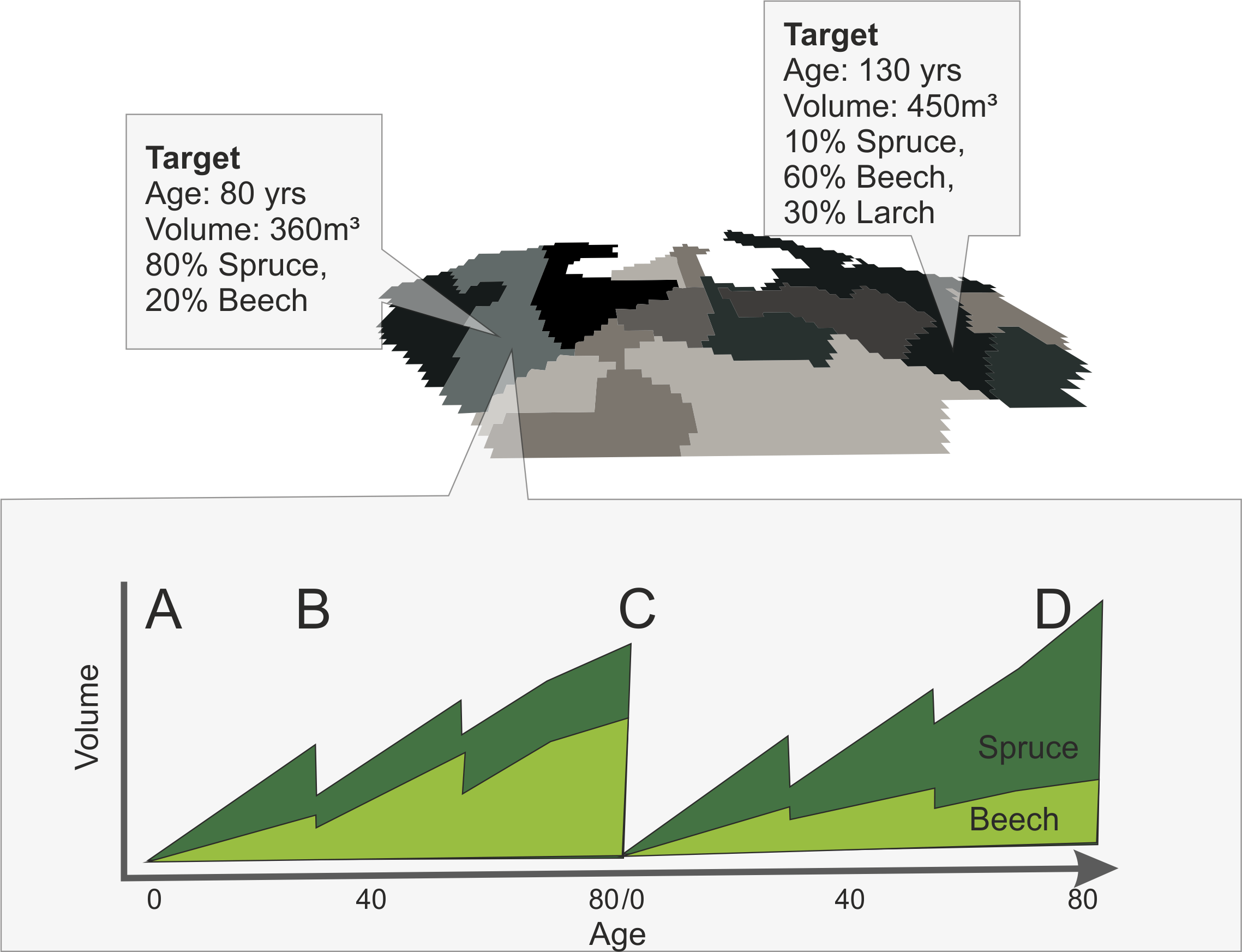
Figure 1 (upper panel) shows an example landscape with a number of “stand”-polygons. Each polygon can have a number of target attributes (e.g., age, species shares, growing stock, …). Target variables are derived from available data on the current state of the system (e.g., forest management plans, inventory plots, remote sensing).
For each stand polygon a single stand treatment program (STP) is created based on information past management regimes and the current state of the system (i.e., the initialization target). Such a typical STP for managed forests in Central Europe includes planting, thinnings and a final cut (in addition to a specific activity used internally by the spinup). For instance, the initial planting could plant trees according to the target species shares (A). Note that this happens simultaneously for all stands on the landscape. During the simulation the defined management steps are executed (e.g., thinnings, B). When the dedicated rotation age is reached (C), the state of the forest on the stand is evaluated. A basic evaluation compares for instance the realized timber volume and/or species shares with the respective target values and calculates a “similarity score”. When the targets are not met, the management plan for the next rotation can be altered. In this example, the simulated share of spruce was lower than the observed spruce share, indicating that spruce was likely favored by past management, either by planting (and thus increasing the initial share of spruce) (C) or by favoring spruce via selective thinnings. The thus modified STP is then used for the next rotation (D). At the end of the rotation the iterative process of evaluation and modification is repeated. Whenever the simulated forest state is more similar to the target state (as indicated by a higher similarity score), the full state of the stand is stored within a snapshot data base, potentially overwriting previously saved states. Please note, that this process is executed for all stands of the landscape in parallel. The final step of the process (after, e.g., 500 years) is for each stand to load the previously saved forest state (i.e., the state that had the highest similarity score relative to the observations throughout the spin-up run) and to create a single landscape scale “composite” from all of these thats, that can be used as the initial state for subsequent simulations. The spinup procedure creates detailed log files which can be further analyzed (see below).
Implementation details
The implementation of the spinup makes heavy use of the Javascript interface of iLand and the built-in forest management engine. The components are:
- iLand: the model includes the forest management engine and provides a Javascript interface (API)
- spinuplib.js: a little Javascript library that contains a number of helping functions / classes
- spinup.js: the bits of Javascript logic which are specific to a project. Note that the split between library and user code is rather soft and will likely evolve over time (and more spinup applications)
What follows is a brief discussion of the parts of the provided example code that need to be adapted for a new application (function names refer to the example source code in ‘spinup.js’:
- definition of the target values and loading the target values in iLand (see loadTargets())
- definition of the standard management activities and the standard management program (see buildProgram(), and the ops-object with activities)
- Calculation of a ‘similarity score’ (runEvaluator()). This depends on the target variables; the library contains a function to calculate the Bray-Curtis index (expressing similarity of tree species shares).
- Definition of “updates” to the STP; the script contains an update of species shares during planting, but additional modifications may be added (see buildProgram() for an example)
- Adapting the analysis R script: the script reads the log file created by the spinup and creates a neat PDF document showing the progress of the spinup, and results for single stands and the whole landscape.
Helpers
The following helper functions/classes are available in spinuplib.js:
- DBHDist: holds a landscape-level DBH distribution that always reflects the current state of the spinup snapshot database (and not the current state in the simulation model). This DBH distribution can be compared to measured DBH distributions (e.g., from sample plots)
- Logger: a helper class to write log messages; the R script parses the log files
- Snapshot: a class encapsulating the stand-wise saving/reading of forest state information to the spinup snapshot database. Currently, the system needs a table (‘ru_file_list’) that lists for each stand the Ids of resource units that are covered by the stand (note that this might change in the future). During testing, the actual saving of the snapshot can be omitted (which saves a lot of time) by out-commenting the two lines in the Snapshot.save() function.
- updatePlantingTarget(), calculateSpeciesProbabilities(): functions that change the species shares in planting (updatePlantingTarget()), and define species selectivity during tending (calculateSpeciesProbabilities()).
Creating a final "snapshot"
The final steps of creating a spinup are:
- run the spinup (during the simulation the "stand snapshot database" gets filled with saved stands and carbon values)
- create the spinup project again (usually without trees). Then load the content of the stand snapshot database. This can be done using Javascript (either use the loadAll function of the Snapshot object (spinuplib.js) or use the iLand API functions directly (loadStandSnapshot, loadStandCarbon). Check the log output if the operation was successful.
- now you have the landscape populated with the trees (and saplings and carbon pools). You can now create a regular snapshot (saveModelSnapshot). The thus created snapshot can be used to initalize iLand (note that this snapshot does not depend in any way on the stand polygons that were used during spinup).
Examples
Kalkalpen
Targets are here defined as the species-specific stand volume and age (each stand may contain several age classes to account for multilayer structures) as well as the vertical structure obtained from LiDAR data (optional).
In a spin-up library (spinuplib.js) we defined relevant functions for the spin-up procedure such as the computation of a Bray-Curtis-Similarity Index to compare the simulated with the target species composition, and the function to save stand snapshots. Next, we defined species and site specific planting, tending, thinning and harvesting activities (stand_init_test.js). Initially, plantings correspond to the relative target volume per species in each stand. If the Bray-Curties Index is >0.2 at the end of the rotation period, iLand autonomously adapts planting activities, aiming to derive a species composition closer to target values. Additionally, species fractions and sapling height can be adapted manually. Moreover, we differentiated planting patterns with shade-intolerant species planted in groups while shade-tolerant species were planted everywhere on the stand (excluding already occupied areas from shade-intolerant species) in order to improve performance and patterns of shade-intolerant species. Tending and thinnings are specified by the stand age at which the activity is conducted, the amount of timber removed (absolute or relative), the minimum dbh for tree removal, and the relative share of trees to be cut per stratum (e.g., in order to differentiate between thinnings from below and from above). The rotation length is defined by the target stand age. The target stand age can be differentiated per tree species and/or per stratum (e.g., if a stand contains more than one age class, only the oldest age class is cut when the rotation length is reached). Different stand treatment programs (STPs) might be defined to refine plantings, tendings, thinnings and harvests (e.g., to vary the number of cohorts planted for one species over elevation). A combined index including the Bray-Curties-Similarity Index and the relative difference from the target volume determines whether a stand is saved at the end of each rotation or not, i.e., if this index was higher in a previous stand snapshot, its information about vegetation and soil properties will be overwritten. After the spin-up period, the stand snapshot databased has to be opened in iLand (command: Globals.loadStandSnapshot() ) to reassemble stands to the total landscape again which then can be saved as landscape snapshot (command: Globals.saveModelSnapshot() ).
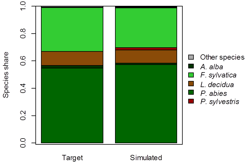
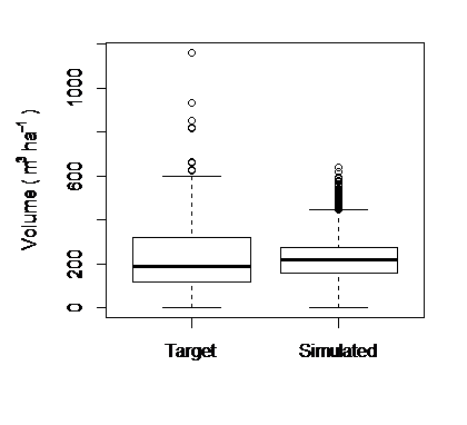
For a current study of Kalkalpen National Park (KANP), our aim was to initialize the historic landscape based on forest management and planning data (stand level data) from archives for which we had information on species composition and age classes per stand at the beginning of the 20th century (init_cent_agg.csv), but we were lacking data on tree height and position, regeneration as well as carbon pools. For an initial estimate of belowground carbon pools, we used the data of KANP formerly derived by Thom et al. (2017) for the year 1999. As this was just a rough estimate, we set a condition to prohibit saving of stands within the first 100 years of the simulation in order to receive meaningful belowground carbon pools, however, any initial estimate may work – the higher the distance from the true value is, the more years should be simulated without saving carbon pools. We started with a landscape from bareground with reduced nitrogen pools and simulated it for 1000 years into the future under historic climate conditions. Further, the simulation included a forest management approach typical for Austria during the turn of the century with low-intensity thinnings from below, and clear-cuts at the end of the rotation period (sensu Österreichischer Forstverein 1994). In total 2079 stands were simulated and saved, and subsequently reassembled to the landscape representing the state of forest vegetation in 1905. Our evaluations indicate a good match between simulated and target tree species composition (Fig. 3) as well as simulated and target volume (Fig. 4) on the landscape.
Stubaital
The spinup example for the Stubaital comes with the full code:
- spinuplib.js: The spinup library
- spinup.js: the user code part
- analysis.R: the R script to evaluate and analyse the log messages
The files are attached to this wiki-page.