spread algorithm

The fire spread algorithm is implemented using a cellular automaton approach. Fire spreads from burning cells to neighbor cells with a transfer probability which depends on wind direction and slope. The estimated fire spread distances established by Keene et al therefore need to be translated into probabilities.
The main principle of the spread algorithm is shown in Figure 1. For each currently burning cell a transfer probability for the 8-neighborhood is estimated (Figure 1, left). A uniform random number (0,1) decides if the fire spreads in the next round (Figure 1, right). Cells burn and spread fire only during one round. If a cell is potentially ignited from more than one cell (Figure 1, right), then the transfer probabilities are stochastically added ( Eq. (1)).

\[\begin{aligned} p_{transit} = 1-\prod (1-p_{i}) \end{aligned} \]

Eq. 1

with p_transit the resulting and p_i the individual transit probabilities.

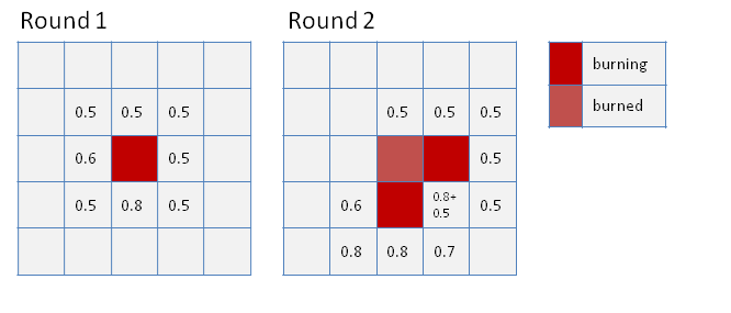
Figure 1: scheme of the spread algorithm.

estimating the probability of spread

The empirical formulas from Keene et al. estimate the metric distance that fire may spread from a burning cell. This distance is translated to the transit probability that results in a 50 per cent chance of reaching the estimated distance. This estimate assumes equal probabilities for each transit on the way (Eq. (2)).

\[\begin{aligned} p_{transit} = 0.5 ^{\frac{d_{spread}}{cellsize} } \end{aligned} \]

Eq. 2

with d_spread the estimated spread distance, and cellsize the pixel size (20 m).

By calculating transit probabilities for each cell, a forest aisle can effectively stop the fire spread. In addition, the local slope characteristics are always used.

Step by step description for each cell-neighbor pair:

• calculate the estimated fire spread distance in the given direction following the formulas described in wildfire
• calculate from that a spread probability (Eq. 2)
• reduce the spread probability by multiplying the rLand factor
• add the probability to burn according to Eq. 1

dynamic fire size calculation

As described here, the size of a fire is estimated from a fire size distribution. An important parameter is the defined average fire size (averageFireSize in the XML file) of the resource unit containing the ignition point. What happens, if the fire spreads (as outlined above) to a neighboring resource with a different defined fire size?
The solution we'd finally came up with, modifies the fire size dynamically while spreading. From the stochastically derived fire size for the start point a ratio is calculated:

\[\begin{aligned} f_{size} = \frac{firesize}{averageSize} \end{aligned} \]

Eq. 3

with averageSize the pre-defined value for a given resource unit.
The total fire size at the nth burning cell is subsequently calculated according to Eq. (4):

\[\begin{aligned} fireSize_{n} = \frac{1}{n} \sum_{i=0}^{n} averageSize_{RU_{n}}\cdot f_{size} \end{aligned} \]

Eq. 4